激活函数们
为什么使用激活函数
因为线性模型的表达能力不够,引入激活函数是为了添加非线性因素。

在没有激活函数的神经网络中,每一层输出的都是上一层输入的线性函数,所以无论网络结构怎么搭,输出都是输入的线性组合。
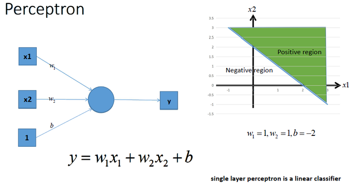
上图中是一个单层感知机。单层感知机能够将空间用直线划分为两个区域,从而获得一种类似二分类的能力。
我们可以通过多个感知机的组合,获得更强的分类能力:
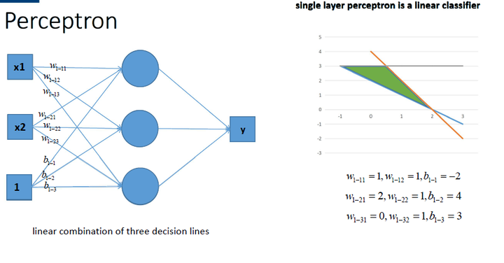
当多个感知机组合时,会在空间内画出多根直线,将空间分成很多份,或是在空间内独立出一个封闭的有限图形。这使得感知机获得了更强的分类能力。
我们来看一下上如的感知机进行组合输出的结果:
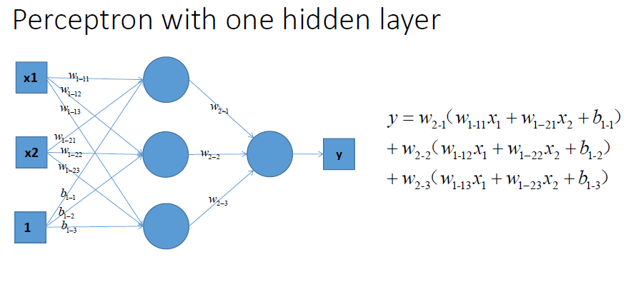
可以看出,不论怎么组合,都是输出都是输入的线性变换,无法做到能够用在空间内画出曲线或是更复杂操作的非线性分类。
常见的激活函数
ReLU函数
ReLU(rectified linear unit)函数提供了一个很简单的非线性变换。给定元素x,该函数定义为$\text{ReLU}(x) = \max(x, 0) $
可以看出,ReLU函数只保留正数元素,并将负数元素清零。为了直观地观察这一非线性变换,我们先定义一个绘图函数xyplot。
import tensorflow as tf
import matplotlib.pyplot as plt

x = tf.constant(range(-8, 8, 1))
out = tf.nn.relu(x)
plt.xlabel("x")
plt.ylabel("reLU x")
plt.plot(x, out)
plt.show()
下图是会上面这段代码绘制出的图形
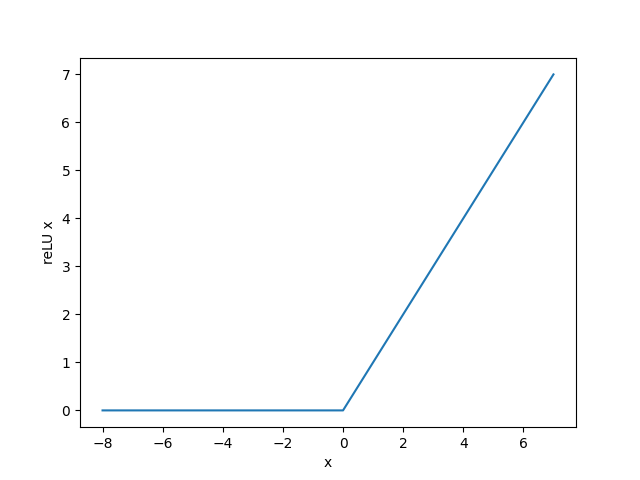
可以看出,该函数定义为 \text{ReLU}(x) = \max(x, 0) $ ,在 $x>0 处函数值为 本身。因此在 处的梯度应该是1。
接下来我们打出它的梯度:
x = tf.Variable(tf.cast(x, dtype=tf.float32))
with tf.GradientTape() as tape:
    y = tf.nn.relu(x)
plt.xlabel("x")
plt.ylabel("(reLU x)\'")
grad = tape.gradient(y, x)
plt.plot(x.numpy(), grad)
plt.show()
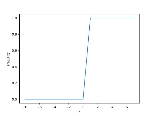
下图是代码打印出的图形:
Sigmoid函数
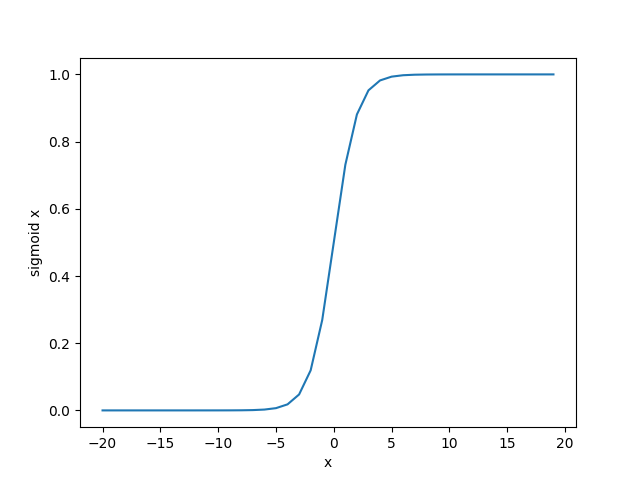
sigmoid函数可以将元素的值变换到0和1之间:
sigmoid函数在早期的神经网络中较为普遍,但它目前逐渐被更简单的ReLU函数取代。在后面“循环神经网络”一章中我们会介绍如何利用它值域在0到1之间这一特性来控制信息在神经网络中的流动。下面绘制了sigmoid函数。当输入接近0时,sigmoid函数接近线性变换。
我们绘制sigmoid的函数图像:
import tensorflow as tf
import matplotlib.pyplot as plt

x = tf.constant(range(-20, 20, 1))
x = tf.cast(x,dtype=tf.float32)
out = tf.nn.sigmoid(x)
plt.xlabel("x")
plt.ylabel("reLU x")
plt.plot(x, out)
plt.show()
这段代码绘制的图像如下图:
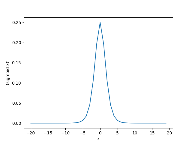
依据链式法则,sigmoid函数的导数为:
下面绘制了sigmoid函数的导数。当输入为0时,sigmoid函数的导数达到最大值0.25;当输入越偏离0时,sigmoid函数的导数越接近0。
x = tf.Variable(tf.cast(x, dtype=tf.float32))
with tf.GradientTape() as tape:
    y = tf.nn.sigmoid(x)
plt.xlabel("x")
plt.ylabel("(reLU x)\'")
grad = tape.gradient(y, x)
plt.plot(x.numpy(), grad)
plt.show()
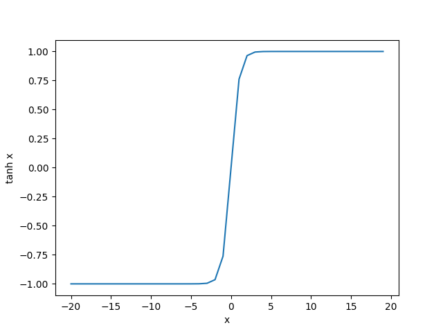
tanh函数
tanh(双曲正切)函数可以将元素的值变换到-1和1之间:
我们接着绘制tanh函数。当输入接近0时,tanh函数接近线性变换。虽然该函数的形状和sigmoid函数的形状很像,但tanh函数在坐标系的原点上对称。
这段代码将会打印tanh的图像:
import tensorflow as tf
import matplotlib.pyplot as plt

x = tf.constant(range(-20, 20, 1))
x = tf.cast(x,dtype=tf.float32)
out = tf.nn.tanh(x)
plt.xlabel("x")
plt.ylabel("reLU x")
plt.plot(x, out)
plt.show()
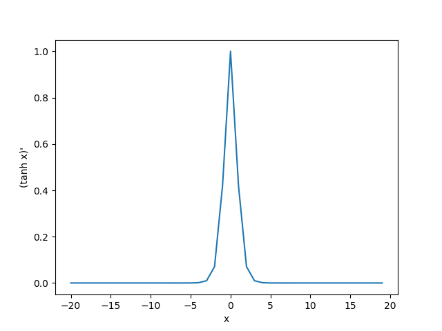
老规矩打印tanh梯度的图像:
x = tf.Variable(tf.cast(x, dtype=tf.float32))
with tf.GradientTape() as tape:
    y = tf.nn.tanh(x)
plt.xlabel("x")
plt.ylabel("(reLU x)\'")
grad = tape.gradient(y, x)
plt.plot(x.numpy(), grad)
plt.show()